Local Density versus k-means Performance on KDD 99 dataset
18 Aug 2014I did a comparison between two clustering methods. One method is from a recent science paper called Clustering by fast search and find of density peaks and the other is k-means. Based on visual inspection and clustered result’s summary, the local density wins. However, in terms of computation complexity and memory spending, k-means seems to be better at manipulating big data set than local density method.
Cluster by local density
Rodriguez and Laio hypothesized that cluster centers are recognized as local density maxima that are far away from any points of higher density. Then they defined two metrics and to measure the cluster’s above attributes (local density and distance to another cluster of higher density) and pick the observations that have both larger and as cluster centers. Please refer to the paper or my previous summary post for details.
K-means
K-means randomly initializes observations as the center cluster. Then it iterates the following assignment and update processes and stops when assignments no longer change or iteration number goes beyond predefined iteration threshold.
| Variable | Definition | Type |
|---|---|---|
| Observation vector | Feature Vector | |
| Observations cluster contains at th iteration | Set | |
| th cluster center at th iteration | Feature Vector |
Initial step: Randomly pick observations as cluster centers (or cluster means) . Cluster mean is defined as the average of all observations in that cluster:
where counts the number of observations in set .
Assignment step:
where is what cluster contains at th iteration. The above formula tells us to assign observation to its nearest cluster center .
Update step: Calculate new mean or update cluster center after the assignment step.
The algorithm can only converge to a local minimum, since the optimization problem k-mean tries to solve is NP hard. k-means tries to find the optimal sets that minimizes the within-cluster sum of squares. However, we can run k-means many times and pick the best one that minimize the following.
Comparison on KDD99
KDD99 is a network security dataset. I used the 10 percent training subset which is of dimension . I disregarded all categorical variables, since they bring some trouble in my following data visualization.
For the local density method, I minorly revised the matlab code provided in their paper since I didn’t want to calculate the halo of cluster (I think the cluster halo or outliers are defined as the controversial points between clusters that can be assigned to two or more clusters. In their original code, they assign a point as cluster halo if its density is below the cluster center’s neighborhood average density). Because the method needs to calculate observations’ pairwise distance, it has to save at least numbers for the distance matrix . However, matlab’s maximum memory for storing a vector is 677 MB in a 32-bit system. I have to give up by randomly sampling only 10K of that subset and my comparison is based on a subset with sampling seed 2014. You can set the seed and reproduce my result exactly via:
rng(2014);
idx = randsample(size(M,1), 10000);
For the k-means part, I used matlab’s build-in kmeans function and replicated the algorithm for 1000 times to select the best solution.
Data Visualization
I used PCoA to reconstruct the spacial relationship between different points by their distance matrix . In matlab, you can realize PCoA using cmdscale, pass the distance matrix to it and it will return a reduced dimension matrix and ’s eigen values. If the first 2 eigen values are comparable larger than the rest, we can safely preserve large information for visualization by the first 2 vectors in matrix while discarding the minor one. You can also use mdscale which preforms nonmetric multidimensional scaling on the dissimilarity matrix (distance matrix is one type of dissimilarity matrix).
>> [Y,eigvals] = cmdscale(D);
>> eigvals(1:4)
ans =
1.0e+03 *
1.9623
1.3507
0.2575
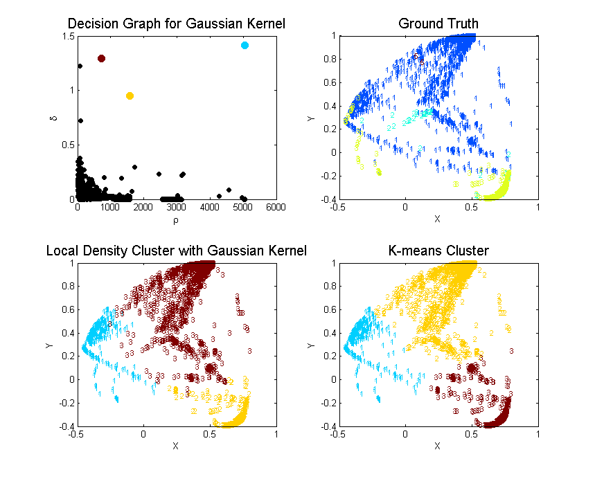
0.1995Since and are much larger than the rest, we can visualize using the first two vectors in . All data points are colored by their ground truth and there are five categories summarized in the table below.
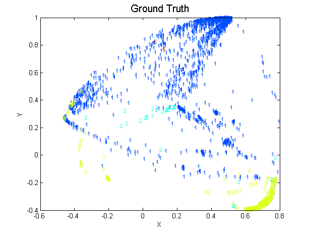
| Code | Type of attack | Number | Color |
|---|---|---|---|
| 1 | normal | 1984 | Blue |
| 2 | probe | 73 | Green |
| 3 | denial of service (DOS) | 7941 | Yellow |
| 4 | user-to-root (U2R) | 0 | NA |
| 5 | remote-to-local (R2L) | 2 | Red |
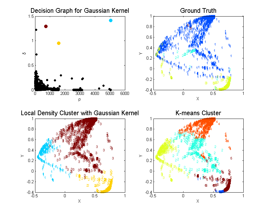
Local Density
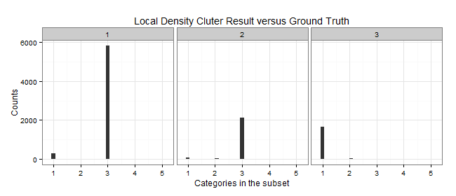
| Cluster | Color | Elements | C1 | C2 | C3 | C5 | Purity | MDtC |
|---|---|---|---|---|---|---|---|---|
| 1 | Blue | 6107 | 289 | 1 | 5817 | 0 | 0.9525 | 2.75 |
| 2 | Yellow | 2230 | 58 | 48 | 2124 | 0 | 0.9525 | 3.24 |
| 3 | Red | 1663 | 1637 | 24 | 0 | 2 | 0.9844 | 5.11 |
| Total | 10K |
K-means: K = 5
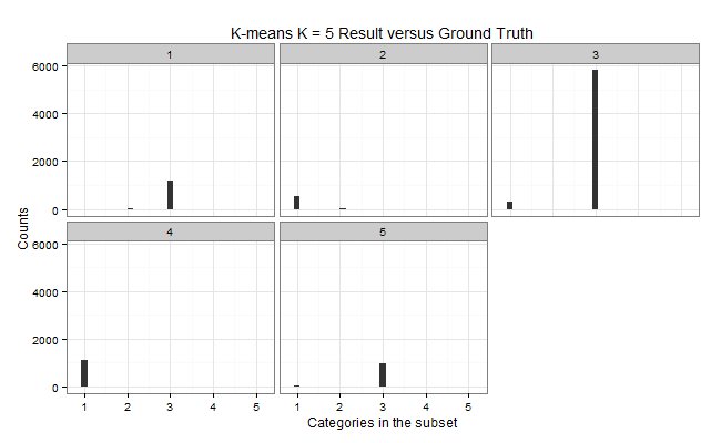
| Cluster | Color | Elements | C1 | C2 | C3 | C5 | Purity | MDtC |
|---|---|---|---|---|---|---|---|---|
| 1 | Blue | 1200 | 2 | 29 | 1169 | 0 | 0.9742 | 1.76 |
| 2 | Green | 561 | 537 | 24 | 0 | 0 | 0.9572 | 4.46 |
| 3 | Yellow | 6105 | 287 | 1 | 5817 | 0 | 0.9528 | 3.03 |
| 4 | Orange | 1099 | 1097 | 0 | 0 | 2 | 0.9982 | 3.77 |
| 5 | Red | 1035 | 61 | 19 | 955 | 0 | 0.9227 | 3.81 |
| Total | 10K |
K-means: K = 3
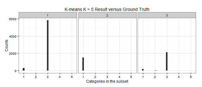
| Cluster | Color | Elements | C1 | C2 | C3 | C5 | Purity | MDtC |
|---|---|---|---|---|---|---|---|---|
| 1 | Blue | 6117 | 294 | 6 | 5817 | 0 | 0.9509 | 3.69 |
| 2 | Yellow | 1543 | 1522 | 19 | 0 | 2 | 0.9864 | 4.73 |
| 3 | Red | 2340 | 168 | 48 | 2124 | 0 | 0.9077 | 3.84 |
| Total | 10K |
Performance Comparison
Since the unsupervised learning is evaluated by how well they grouped the ground truth labels into clusters. We can define the purity of the algorithm by . As we can see from the above Purity, cluster by local density beats k-means by large.
It is somewhat difficult to calculate attack type wise precision such as DoS, probe detection rate. Since unsupervised learning lacks important labeling information, its performance in multiple classification problem should be considerably bad than some supervised learning methods for example random forest, svm etc. However, it is more essential for us to detect the attack from the normal than to further know its type. Life would be a lot of easier, if we can group all different attacks into one and treat the above as bi-classification problem.
After observing the ground truth visualization, we can easily find that the normal traffic (blue points) are more spread out than the attacks. We can simply measure the level of spread by calculating the max sum of distance of all points to its group’s center. The maximum sum of distance to center is defined as
where denotes the th dimension of vector , is the center of group and as the group ’s maximum sum of distances. Although might sound less straight forward than the sum of dimensional-wise variance, I think is more computational saving.
Anyway after assigning the maximum ’s group as normal cluster, we now can calculate the following performance table:
| Method | Precision | False Positive Rate |
|---|---|---|
| Local Density | 0.99676 | 0.17490 |
| K-means K = 5 | 0.99701 | 0.72933 |
| K-means K = 3 | 0.99738 | 0.23286 |
In the case of false positive rate, local density method wins. But the false positive rate is such high that unfortunately it is of little practical usage.
Revised OMP
Use ’s weight as voting for labels and break the loop if residual’s L2 norm is less than some threshold.