In the machine learning literature, many learning algorithms’ performance are hampered by the high dimensionality of the real world data which is also known as the curse of dimension. It is of utmost interest for the researchers to do multidimensional scaling (MDS) and have a vivid insight into the actual structure of the data. Dimensional reduction tries to find the intrinsic dimensionality from the data. Suppose we have a high dimensional data with a feature space . Dimensionality reduction techniques map into a lower dimensional space and, meanwhile, keeps as much information as possible. One way to understand these techniques is to treat high dimensional data in a latent space as a stochastic process and then map the data to lower dimensional spaces such that the structure of data is maintained.
Over the last decades, there are many good algorithms purposed to reduce dimensions. Some of them focus on maintaining local structures, such as ISOMAP [5] (Tenenbaum et al., 2000), Local Linear Embedding [4] (Saul et al., 2006) and Maximum Variance Unfolding (MVU; Weiberger et al., 2004) while others look at variance maximizing, like PCA (Goldberger et al., 2005), MDS (Young et al. 1938) and autoencoder (Hinton et al., 2006). However, for non-parametric manifold learners, the main limitation is that they don’t provide a parametric mapping between the data points. For spectral techniques, this out-of-sample extension can be realized by some approximations. But they usually need to handle a broader range of cost functions, which may cause computational problems.
This report aims at the rationale behind SNE and tSNE and validating their performance. The report is structured as follows. Section 2 entails SNE. In particular, we will exam how SNE define similarity metrics, construct cost function and optimize the function. Section 3 begins with the drawbacks faced by SNE and discusses what changes tSNE makes to alleviate the problems. Section 4 provides a detail comparison between tSNE and other MDS methods on four simulation and two real datasets. Finally, we conclude that tSNE is among the successful non-parametric MDS methods and recommend researcers adding it to their MDS toolbox.
Stochastic Neighbor Embedding (SNE) [6] maps the data points in high-dimension space , where into observable low-dimension space , or . SNE converts the the high dimensional Euclidean distance between data points into conditional probability for the similarity measurement. Or for any , we define conditional probability in Eq (↓) that would pick as its neighbor if the neighbors were picked up in proportion to the Gaussian density centered at . Since we only care about pairwise similarity, is set to .
Similar for any , we extend the same definition to the mapped lower dimension. is set to as .
Our aim is to find a mapping such that is a good approximation of . Since both and are some measurement of the probability, we can naturally use cross-entropy or Kullback-Leibler divergence to minimize the information lost those two.
Notice that the lost function defined in Eq (↓) is non symmetric such that use small to model large is largely penalized than the reverse. In other words, the SNE cost function tends to persevere local structure and leads to the “crowding” problem.
The last parameter to determine is the defined in Eq (↓). Because induces a probability distribution whose entropy increases as increases and the density of variates with individual data point, therefore each data point should have its own . SNE performs a binary search for that produces a with a fixed perplexity defined by the user.
where is the Shannon entropy of defined as
The final step is to minimize the cost function in Eq ↓. We take the derivative with respective to each mapped point and then use Gradient descent.
A momentum term (a decaying sum of previous gradients) is added to the update function to expedite the process.
Although SNE sounds like a good visualization approach, its performance is hindered by the difficult optimization function and the “crowding” problem. The cost function in is hard to optimize in two ways: first we have to determine many parameters such as , perplexity, before the actual optimizing process; second the optimization problem is non convex such that SNE is easily subject to local minimum if some ameliorating action is not taken.
The “crowding” problem is due to the fact that two dimensional distance cannot faithfully model that distance of higher dimension. For example, in 2 dimensions we can find 3 points (an equilateral triangle) that are mutually equal distance but in 3 or dimensions the number of points with such property can be 4 (an equilateral tetrahedron) or . In other words, the area of 2-dimension map available to accommodate mapped points is not large enough for “closed” data points in high-dimension. Since SNE’s non-symmetric metric tends to preserve local structure, SNE makes the “crowding” problem even worse.
t-Distributed Stochastic Neighbor Embedding (tSNE) employs symmetric similarity metrics and heavy tail distribution in the in the low-dimensional space to alleviate the above drawbacks. The symmetric metrics is introduced as Eq (↓) and (↓).
However, Eq (↓) has one additional problem when there are outliers in the extreme high-dimension space. If a data point is an outlier, then all pairwise distances are large for . Then as , converges to , and has little effect on the cost function. An alternative way is taking the average of two conditional probability and as in Eq (↓). But for fast computation definition of Eq (↓) is used, if is not that large.
The lost function in Eq (↓) naturally changes to Eq (↓).
Student t-distribution with one degree of freedom is employed in tSNE or Eq (↓) is replaced by Eq (↓). This change not only allows moderate distance in high-dimension to be faithfully modeled by a larger distance in the low-dimension map but also is much faster to evaluate since it does not involve an exponential term as Eq (↓). The theoretical support for this change is that Student t-distribution is an infinite mixture of Gaussians.
Now the gradient of Lost function becomes
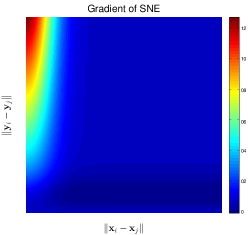
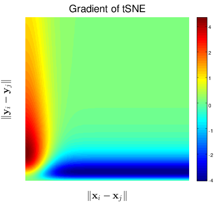
Figure 1↓ shows the gradients as a function of and for the SNE and tSNE. The negative values of the gradients represent an increase in the loss function or a repulsion between two mapped points while the positive values represent an attraction. Notice that SNE’s attraction in Figure a↓ when using small to model large is just less than the reverse but tSNE provides a repulsion force to push and apart. It is the repulsion induced by the symmetric metric and heavy tail t-distribution of that makes tSNE successful in handling the “crowding” problems.
(a) Gradient of SNE
(b) Gradient of tSNE
Figure 1 Comparison of Gradients of the Loss functions
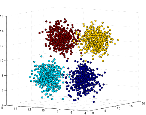
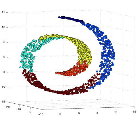
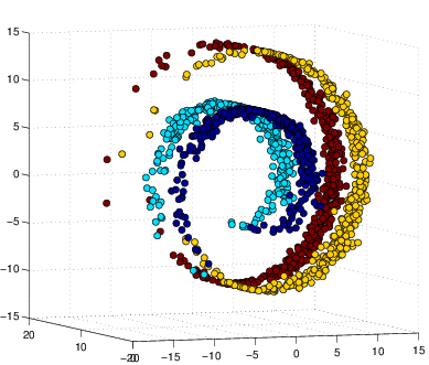
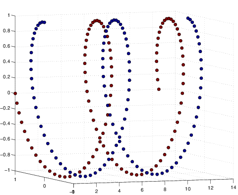
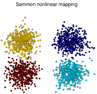
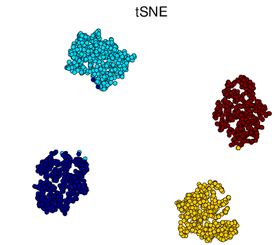
For performance comparison among different visualization methods, we simulated four types of datasets with different statistical distributions. Shown in Figure 2↓, the simulated types are Gaussian mixture, Swiss roll, double Swiss roll and Spiral respectively. For Gaussian mixture data, 4 normal distributions with different mean vectors but the same identical covariance matrix are used for generating and the colors of the data points in Figure a↓ represent their actual labeling. For the Swiss roll data, their color labels are generated by hierarchy clustering with the local constraints [3]. And the double Swiss roll data and their labels were downloaded via this website [A] [A] http://people.cs.uchicago.edu/~dinoj/manifold/swissroll.html.
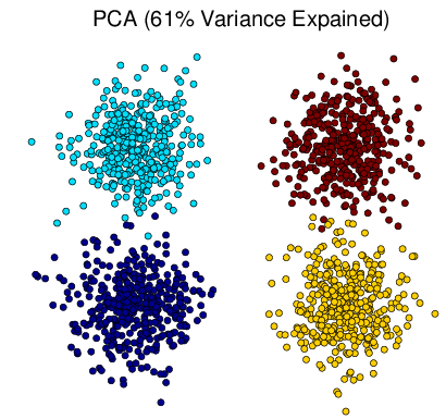
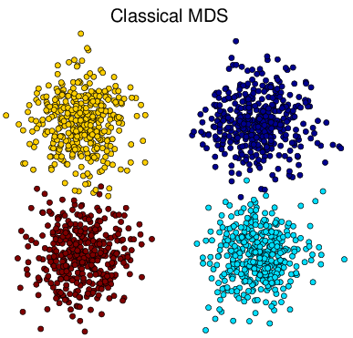
Figure 3 Visualization of Simulated Gaussian Mixture Dataset Results in 2d.
Figure 3↑ shows that all methods successfully obtain the structure of the original Gaussian mixture dataset in Figure a↑ and tSNE is better to group the data points into their relevant clusters than others. Notice that some points are wrongly assigned by tSNE but if we take a look at the original 3d distribution from Figure a↑, those are confusing points within the boundary of two clusters.
Figure 4 Visualization of Simulated Swiss Roll Dataset Result in 2d.
Again all MDS methods successfully attain the internal structure of the original data in Figure b↑. It is interesting to note that tSNE doesn’t preserve the Swiss structure in 2d and assigns some data points wrongly. Since tSNE depends on the conditional probability for similarity metrics other than the traditional pairwise distance matrix, such a distortion of structure can be reasonable and quite acceptable if the researcher just wants to detect the internal relationships between datapoints. The missclassification issue can be related to either a non suitable perplexity (40 in our case) or the bad performance of hierarchical clustering as we don’t have the ground truth labels.
Figure 5 Visualization of Simulated Double Swiss Roll Dataset Result in 2d.
This time PCA and CMDS fail. tSNE performs even better than Sammon despite failing to keep the double Swiss roll structure. This example illustrates the linear techniques including PCA and CMDS that focus on keeping the low-dimensional representations of dissimilar data points far apart fail when high-dimensional data lie on a non-linear manifold as Figure c↑. In high-dimensional setting, it is more important for a MDS to keep the low-dimensional representations of very similar data points close together.
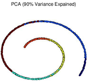
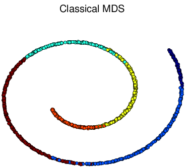
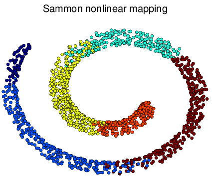
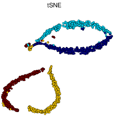
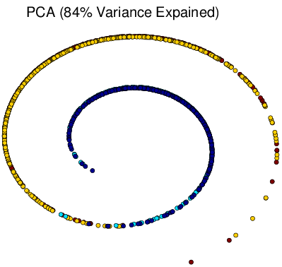
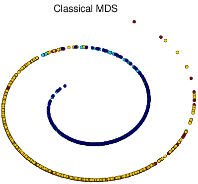
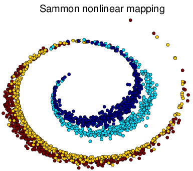
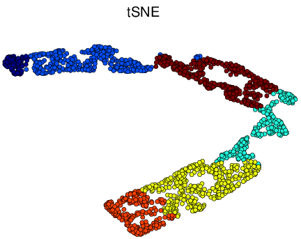
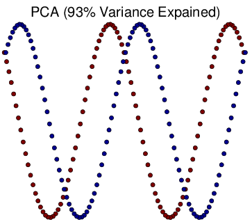
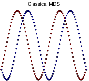
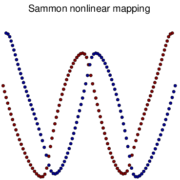
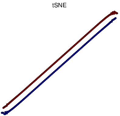
Figure 6 Visualization of Simulated Spiral Dataset Result in 2d.
tSNE successfully attain the structure this time while others fail. Similarly as discussed above, for high-dimension data lying on a non linear manifold, it is more important to keep similar points together. Figure d↑ shows a “Stochastic” property of tSNE that once the data point in the Markov process converges to a stable state, it gets stuck in that state.
In the following, we compared the PCA and tSNE’s performance on two real high dimensional datasets. The first real dataset is the training data of STAT 640 data mining competition [1] which is a 66.3% subset of the full Human Activity dataset [2]. The training data contains a data matrix of size 6,831 observations by 561 features and 20 subjects comprise the subset. Each observation is uniquely assigned with a class activity label coded from 1 to 6. The actual number of observations of each activity and the activity labels are coded in Table 1↓.
Code
Activity
Observations
Type
1
Walking
1108
Dynamic
2
Walking Upstairs
1025
3
Walking Downstairs
928
4
Sitting
1192
Static
5
Standing
1263
6
Laying
1315
Table 1 Activity Labels and Relevant Codes
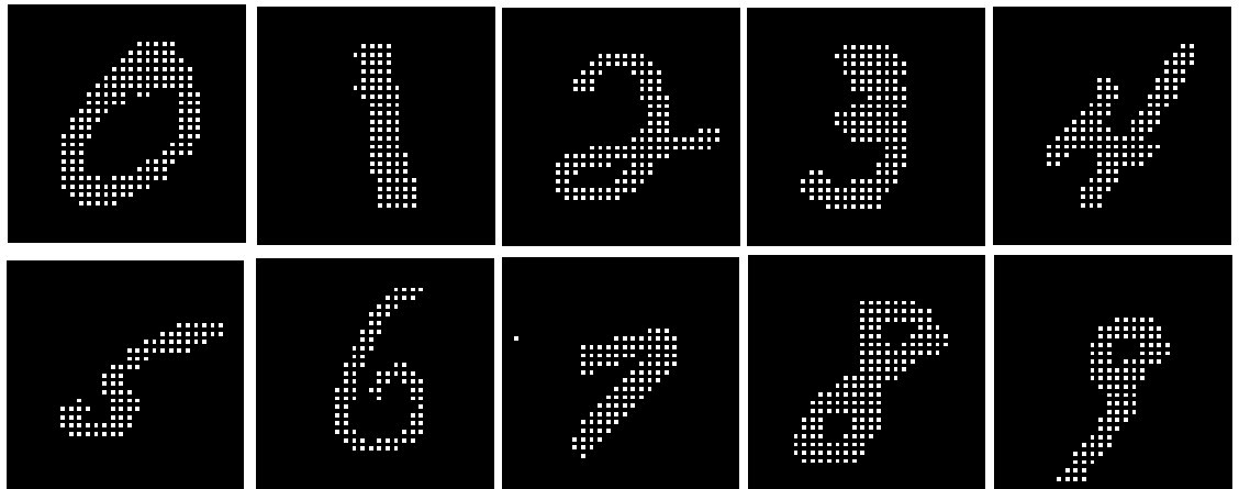
Another real dataset is the training set of MNIST handwritten digits data containing a data matrix of 60,000 examples by 784 variables. Each observation is a “normalized” black and white image of certain digit. Sampled digits from 0 to 9 can be referred by Figure 7↓. For better visualization, we magnify the resolution of each digit but the original resolution is or a vector of size in dimensions.
Figure 7 10 samples from MNIST digits dataset.
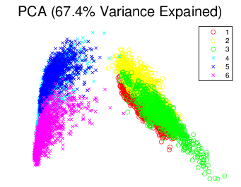
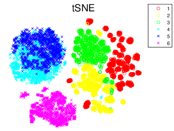
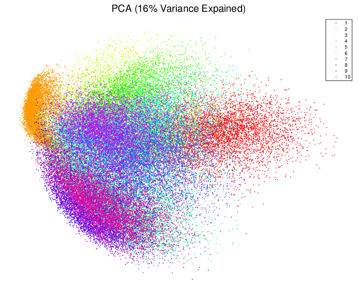
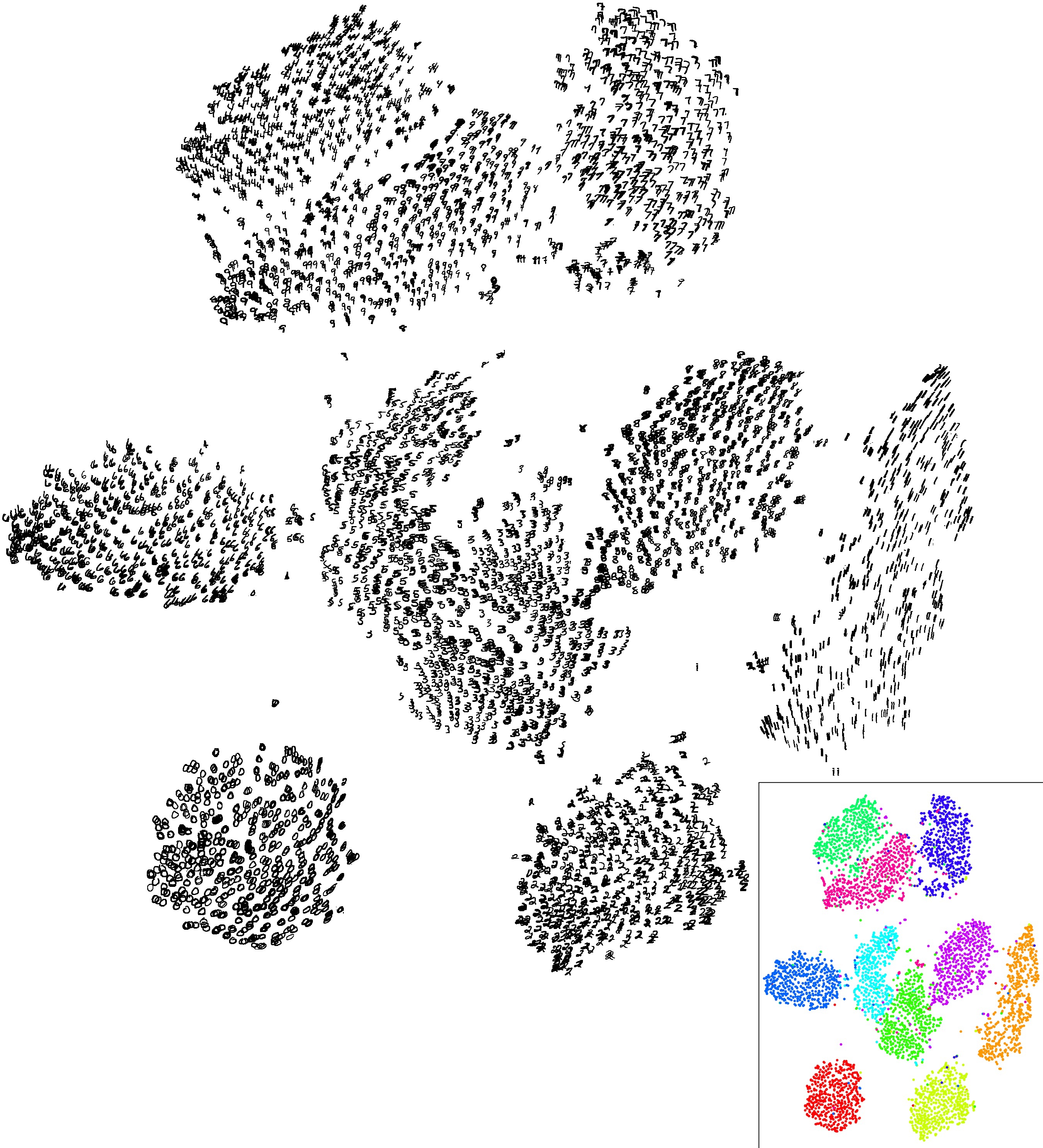
In Figure 8↓, we show the results of the experiments with PCA and tSNE on Human Activity dataset. The results reveal strong performance of tSNE over PCA. In particular, PCA only detect the two main clusters namely 1, 2, 3 as the dynamic pattern and 4, 5, 6 as the static one but tSNE does a considerable better job in separating 1, 2, 3 and 6 into their sub clusters. Although there are some salient overlapping between group 4 and 5, the two clusters, sitting and standing, are seriously mixed up such that even the advanced classifiers such as random forest or support vector machine can not distinguish them well. For the digits data in Figure 9↓, PCA produce little insight to the data with large overlaps between the digits classes but tSNE construct a mapping where we can easily see each clustering in their relevant colors shown in Figure b↓. Although some digits are clustered with the wrong classes, but most of them are distorted digits and quite hard for the human to identify.
In this project we provide details about the rationality of SNE namely its asymmetric conditional probability similarity metrics, cross entropy cost function, non convex optimization problem and its two drawbacks. Then we focus on two alternations tSNE makes to ameliorate crowding and optimization problem by the symmetric join probability and the heavy tail t-distribution in .
Then we compare some MDS methods such as PCA, MDS, non-linear Sammon and tSNE on several simulation and real datasets. It turns out that tSNE always attains better solution than the others. We realize that for data lying on non-linear manifold in high-dimension keeping the similarity data points together is more important than pushing dissimilarity points apart. And the Markov process of mapped data points make tSNE more Statistical reasonable.
One addition drawback for tSNE is that it doesn’t obtain a parametric mapping function. You have to redo the computation when applying to new dataset. However, as an efficient non-parametric MDS methods, tSNE indeed provides an alternative to PCA and the other MDSs to help you gain new insight into your high-dimension data.
[2] Davide Anguita, Alessandro Ghio, Luca Oneto, Xavier Parra, Jorge L Reyes-Ortiz. A public domain dataset for human activity recognition using smartphones. European Symposium on Artificial Neural Networks, Computational Intelligence and Machine Learning, ESANN, 2013.
[3] Ian Davidson, SS Ravi. Agglomerative hierarchical clustering with constraints: Theoretical and empirical results. In Knowledge Discovery in Databases: PKDD 2005 . Springer, 2005.
[4] Sam T Roweis, Lawrence K Saul. Nonlinear dimensionality reduction by locally linear embedding. Science, 290(5500):2323—2326, 2000.
[5] Vin D Silva, Joshua B Tenenbaum. Global versus local methods in nonlinear dimensionality reduction. Advances in neural information processing systems:705—712, 2002.
[6] Laurens Van der Maaten, Geoffrey Hinton. Visualizing data using t-SNE. Journal of Machine Learning Research, 9(2579-2605):85, 2008.