With the wide spread of smartphone popularity and the substantial increase in their functionality, there is much effort in attempting to incorporate all of the features to assist in predicting human activities. With all the additional features to basic telephony, the variety of sensors installed in smartphones can be a powerful tool in Activity Recognition. In this project, we will employ smartphone censors data for human activities recognition, with potential applications in the healthcare industry.
The aim of Activity Recognition is to identify actions carried out by any person, given a set of observations of themselves and the surroundings. Data retrieved from embedded inertial sensors within the smartphone, such as accelerometers, can be exploited for such task. By processing these data through different supervised machine learning algorithm, we will be able classify physical activities, such as standing, walking, laying and etc.
This report is structured in the following way. Section 2 entails the methodologies we have employed. In particular, we will examine the theoretical and logic behind SVM, ELM and ELM’s constraint variants. Section 3 contains two ensemble implementation of ELM namely Random Forest and multiclass Adaboost. Section 4 gives a brief introduction to multidimensional scaling technique called tSNE. Section 5 begins with model selection by cross validation or out of bag errors and then compares testing accuracies among different models. Finally, we give the conclusion and our approach to the data mining competition in Section 6.
In this section, we first briefly introduce the theoretical background of SVM and ELM and their optimization problems respectively. Then we extended the basic ELM models to several variants which impose some constraint on the parameters in the first layer. More comparison among SVM, ELM and Constraint ELM and their performance on the testing data set can be found in Section 5.
In 1995 Cortes and Vapnik [1] proposed the Support Vector Machine (SVM) which maps the data from the input space to some feature space through some nonlinear Prior mapping function . In this feature space, constraint optimization is used to find the “optimal” separating hyperplane that maximize the separating margins of two classifies in the feature space. Given a set of training data points where , and . We can mapped the training data point in the input space to some feature space via a nonlinear function . Then the distance between two hyperplane in the feature space is . We maximize the distance by
where is a slack variables introduced to make data points within the margins satisfies the first constraint in Eq (↓) and is non-negative user-specified penalty term which controls the trade off between training error and the margin distance. Using Karush-Kuhn-Tuchker (KTT) theorem, the above optimization is equivalent to the following
provided that the kernel functions satisfies Mercer’s condition. Then the decision function of SVM is
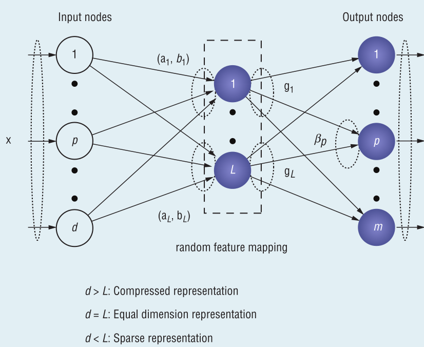
where is the number of support vector and is a sparse representation of the original data matrix or . The SVM can be consider a similar type of Single Layer Feedback Network as illustrate in Figure 1↓.
Guang-Bin Huang and his colleges introduced the extreme learning machine as an SLFN with fast learning speed and good generalization ability (ELM can approximate any target function [3]). Unlike traditional SLFN, the parameters in the hidden layer need not be tuned or fixed once randomly uniform generated. The input data is mapped to the feature space by mapping or where is the activation function for the hidden node as illustrated in Figure 1↑. In Eq (↓), we know SVM can solve bi-classification and SVM is extended to classes classification by One verse One (OVO) or One verse All (OVA). For OVO SVMs are needed and in OVA. However, ELM solves the problem in one model by having output nodes. Then for class the expected output vector is
or only the th element of is one while the others are zeros. ELM is to optimize the training error as well as the norm of the output weights .
where is the hidden-layer output matrix, is the output weights between the hidden layer nodes and the output layer nodes and is the expected output coded as above.
based on KTT theorem whose dual form is
Set the derivative of with respective to , and to zeros. We have
The predicted class label for sample is
Also if the kernel function satisfies Mercer’s condition, we can define the kernel matrix with element . Then Eq (↓) can be reformulated as
and the prediction formula for the Kernel form is the same as Eq (↓).
In previous section, we introduced ELM which maps the original data into the feature space by some activation function (e.g. sigmoid function) whose parameters are randomly generated and then solves essentially a linear system in the second layer. However, it is interesting to investigate whether prediction accuracy on the assessment data set will increase or not, if we add some constraints to the random parameters. The constraints added to the random weights are one of actively research areas in the ELM literature [4, 6]. Since Constraint ELM is claimed to be robust to outliers, here we only present several easily implemented methods for time and space limit.
The constraint difference (CDELM) method utilizes prior “distribution” of two classes. The aim is to constraint the weights to map two classes into positive and negative hyper planes. For observation , it is mapped to and planes by
solve for and , we obtains and where and represent observations from two different classes.
We can generate weight by randomly sample from data matrix and then normalize it (SELM) or sample two data points of different classes and normalize their sum (CSELM). We even can relax the different class constraint and directly normalize the sum of two random sampling (RSELM). There is little statistical support for those constraints but for the competition we tried to believe those will alleviate the possible outliers. However extensive comparison of all the constraint models will be evaluated in Section 5. For a brief reference, the weights and bias are defined in Table 1↓.
Since ensemble is very useful in dealing with overfitting problem and can possibly generate a better model for the testing data set, here we present two ensemble implementations for ELM. Our Random Forest here utilize ELM as week learner. Following Freund et al. [2], we extended the original AdaBoost to multiclass condition. The experiment results of this section is shown in Section 5.
tSNE stands for distributed Stochastic Neighborhood Embedding [5]. Its basic idea is to use conditional probability to define a measure of similarity between data points. Or For any , , define conditional probability that would pick as its neighbor.
For any , same definition extends to mapped lower dimension.
Our aim is to find a mapping such that . Naturally Cross-entropy or Kullback-Leibler divergence is utilized to model the lost between two probability.
Since Eq (↓)’s induces a probability distribution whose entropy increase as increase, an user specific parameter perplexity is introduced to constraint the information. where is the Shannon entropy of defined as . Finally, we can use gradient descent to optimize the cost function in Eq (↓). Or we take derivative in Eq (↓) with respective to each mapped point shown in Eq (↓) and then use monotone Gradient descent in Eq (↓) to update each individual mapped point .
where a momentum term is added to the update function to expedite the descending process. The above is the definition of Stochastic Neighborhood Embedding (SNE) purposed by G. Hinton. They then further changed the condition distribution defined in Eq (↓) to Joint Probability distribution in Eq (↓) and use heavy tail distribution with one degree of freedom shown in Eq (↓).
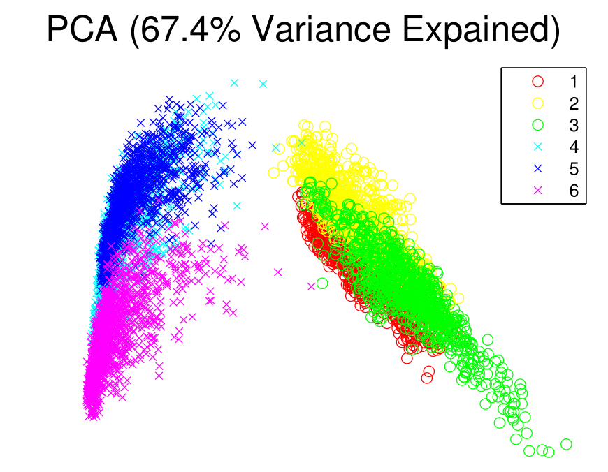
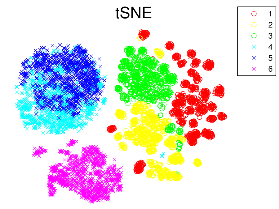
Those changes not only save computational time (exponential term in Eq (↓) is more intensive than the inverse operator in Eq (↓)) but also solves the crowding problem faced in SNE (the area to accommodate similarity points in is not large enough for mapped point ). For more information about the technique detail about t-SNE, please refer to the their paper [5]. Here we present a comparison visualization plots between PCA (or Classical MDS) and t-SNE in Figure (2↓).
(a) PCA
(b) tSNE
Figure 2 PCA and tSNE’s Visualization Result.
We can see tSNE does a better job at visualization than PCA and Group 4 and 5 are such overlapping with each other in t-SNE that we later confirmed some data points between 4 and 5 are hard to separate by either ELM or SVM.
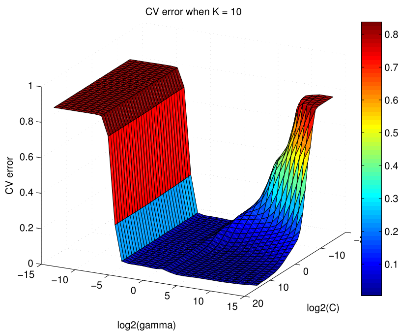
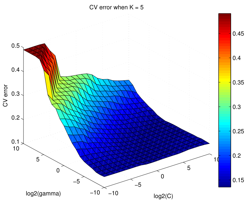
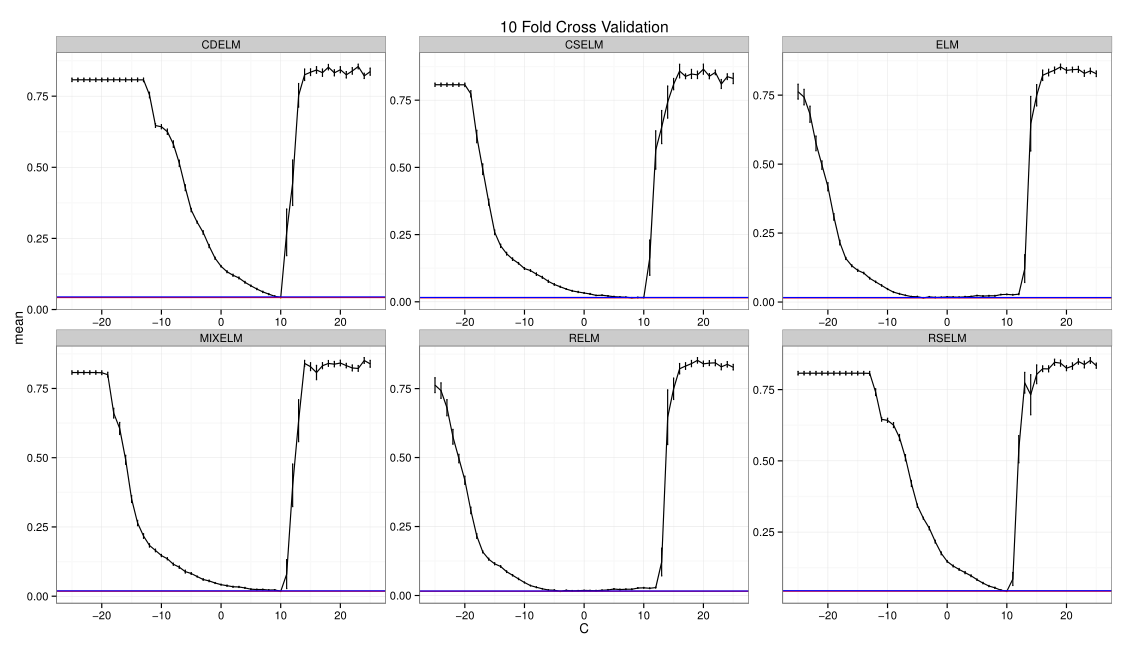
It is important to tune parameters for finding the optimal model with good generation ability and performance on the testing data set. We used minimum Cross Validation errors to select ELM and SVM’s optimal parameters as shown in Figure 3↓ and 4↓. The basic process for Cross Validation is to divide the data set we have into model selection (80%) and model assessment (20%). Further divide the selection data set into folds, and then take turns to build a model using folds to predict on the last fold.
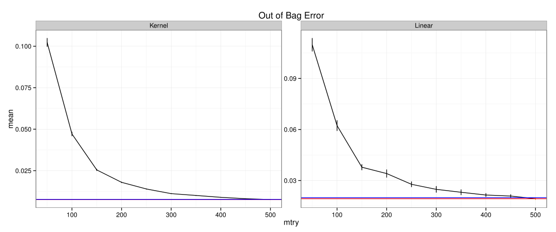
For Random Forest or Bagging, the most convenient way to tune the number of parameters sampled is to use Out of Bag errors or calculate prediction errors on the observations left out from the bootstrap sample. From Figure 3↓ to 5↓, the following parameters in Table 2↓ are used for our model comparison and assessment in the Section 4-2.
Linear Model
Name
SVM
ELM
CDELM
CSELM
MIXELM
RELM
RSELM
Cost
Kernel Model
Name
SVM
ELM
Cost
Random Forest Model
Name
SVM
ELM
mtry
Table 2 Parameter Selected using Cross Validation and Out of Bag errors.
Since we just got the testing data set labels from Dr. Allen, it is interesting to know how those different basic learner perform. Here we present the testing accuracies in Table (3↓) where each model’s parameters are selected in Section 5.1 shown in Table (2↑). However, we don’t have the results for SVM type of Random Forest and Adaboost for time limits. 2000 hidden notes are used in each linear models. Bag number equates to 300 for every random forest and adaboost method.
In this report we compared SVM, ELM and ELM’s constraint versions. ELM outperforms SVM in three ways: First ELM is extremely fast because its time complexity is similar to that of the least squared. Second ELM has better model assessment accuracy as indicated by our competition results. Finally ELM is very easy to implement since it provides an analytical prediction function for the new observations. However, ELM’s theoretical background is even weaker than SVM. Although some researchers pointed out ELM is a deep neural network with infinite layers and it is a biological inspired method, more deep research need to be done to provide a solid theoretical background for the model’s interpretability.
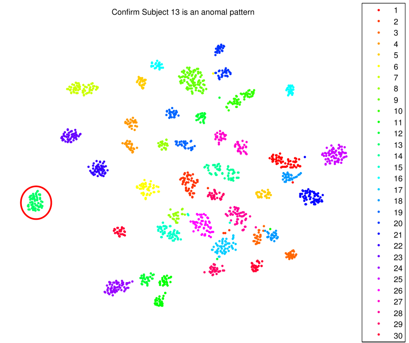
For our final entry, we first iteratively added prediction results returned by kernel ELM. Then we divided our prediction results in to Group 1,2,3 and Group 4,5,6 and separately built two Kernel ELMs. For hard separating classes 4 and 5, we tried to use Random Forest ELM and Adaboost ELM but we gave up those two methods because group 4 and 5 are overlapping seriously enough for any classifier to distinguish them right. Finally, after trial and error we detected testing subject No. 13 as an abnormal walking person in our training set and then used unsupervised methods to recover the label of Subject No. 13 shown in Figure 6↓.
We would like to thank glass and water server at Rice University for providing fast and stable computing power throughout this data mining competition.
[2] Yoav Freund, Robert E Schapire. A desicion-theoretic generalization of on-line learning and an application to boosting. Computational learning theory:23—37, 1995.
[3] Guang-Bin Huang, Lei Chen, Chee-Kheong Siew. Universal approximation using incremental constructive feedforward networks with random hidden nodes. Neural Networks, IEEE Transactions on, 17(4):879—892, 2006.