Crude Oil Price and Volatility Forecasting
20 Dec 2014
Table of Contents
1 Introduction
Nowadays oil price, gold price, currency exchange rates and other macro economic indicators play crucial roles as measures or signals in the world economy. Especially the oil price is always treated most seriously since oil is the blood in the vessels of the economy. Therefore, forecasting the oil price and its volatility has attracted a great amount of attentions from researchers, policy makers and investors. Not mentioning about professionals, people can literately feel the changes caused by fluctuations of oil price in daily lives because of its huge impact. In such sense, we were of most interest and curiosity to investigate the oil price, oil price volatility and dynamic between oil price and other macro economic indicators.
At the same time, the dynamic relationship between these economic indicators are somehow interwound. Besides forecasting the oil price and its volatility we are also interested to discover the dynamic relationship among gold price,currency exchange rate and oil price. We stepped our discovering into three stages. First, we download the data of oil price, gold price and currency exchange rates from Federal Reserve Economic Data (FRED) [A] [A] http://research.stlouisfed.org/fred2, St. Louise Bank in terms of
- Crude Oil Prices: West Texas Intermediate (WTI) - Cushing, Oklahoma;
- Gold Fixing Price London Bullion Market;
- Dow Jones Industrial Average;
- Trade Weighted U.S. Dollar Index: Major Currencies and EU/US Exchange Rate;
- S&P 500 Index;
- Mining Oil and Gas Extraction Employees in Texas;
- Consumer Price Index for All Urban Consumers: Energy;
- Civilian Unemployment Rate.
We took a general look at all the data sets along time axis to have a basic picture intuitively. In addition, we employed Vector Autoregressive (VAR) and constructed pairwise regression between crude oil price and another factor such as gold price, the benchmark index and so on to detect a pool of variables which significantly correlate with the oil price.
On the second stage, we focused on oil price forecasting. We first explored the basic linear time series models such as Random Walk, ARIMA and VAR. We performed routine diagnostics tests to those linear models and made sure they followed their specific assumption. Further we were considering to enhance our forecasting on crude oil price by machine learning techniques. We hence decided to employ non-linear models such as Support Vector Regression (SVR), Multiple Layer Perception (MLP) and Extreme Learning Machine (ELM). Then extensive comparison of forecasting accuracy among those models was conducted based on several error metrics. Our best model for forecasting the oil price is the ELM model.
As for the oil price volatility forecasting, we explored a large range models from
and
family. For
model, we selected the optimal
model with the lowest AIC value. So as we did
model selection. Finally, we nailed down to
as our best choice in oil price volatility forecasting.
2 Oil Price Forecasting
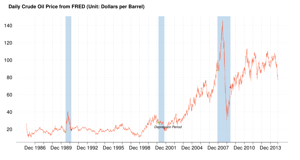
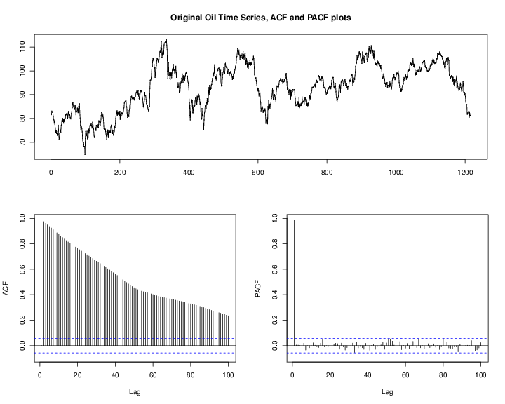
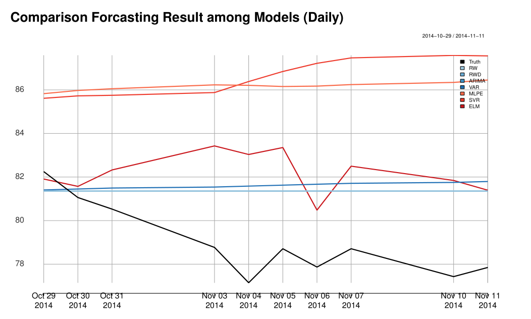
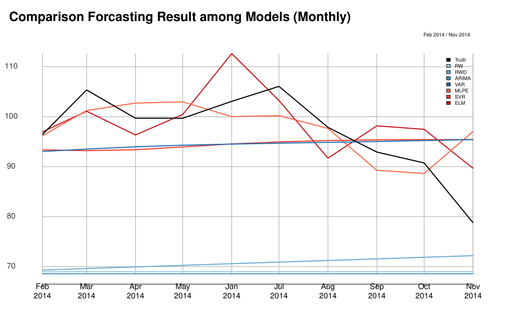
It is an important step to observe the actual oil price time series before building any model. As shown Figure 1↑, the oil price exhibits much variation throughout the history. Especially for those economic regression periods shadowed, the oil price dropped dramatically. For example during the 2008 Financial crisis, the oil price felled off rapidly from 145.31 dollars per barrel, the highest price, to around 30.28. Those extreme fluctuations caused by the financial crisis are unpredictable from our data available, and have seriously bad effect on our models. Therefore we used the observations from 2010-01-01 to 2014-10-28 for building models and 2014-10-29 to 2014-11-11 (10 ahead) for prediction. Since we used some monthly data sets such as Energy Consumer Price Index (ECPI), and Civilian Unemployment Rate (CUR), we shrunk the daily data sets by taking monthly average and separately built another monthly models. The splitting can also be expressed as Training and Testing subset in the Statistical Learning contexts as the below:
Daily Forecasting Models
- Training Range: 2010-01-01 to 2014-10-28 (1258 Observations).
- Testing Range: 2014-10-29 to 2014-11-11 (10 Observations).
Monthly Forecasting Models
- Training Range: 2009-01 to 2014-01 (71 Observations).
- Testing Range: 2014-02 to 2014-11 (10 Observations).
In the following section, we denoted Daily oil price as
and Monthly as
and introduced two types of models to forecast Oil Price. We considered the random walk, ARIMA and Vector Autoregressive (VAR) models as the group of linear time series models and Support Vector Regression (SVR), Multiple Layer Perception (MLP) and Extreme Learning Machine (ELM) as anther group of non-linear models. Then we did extensive comparison of their forecasting power by several important error metrics. Because of space limits, we put all the diagnostics plots of this section to the Appendix.
2.1 Linear Models
The ACF plot of the original oil price time series in Figure 6↓ indicates that the oil price has strong serial correlation and shows the pattern of a unit-root nonstationary time series. We should take a first order difference of
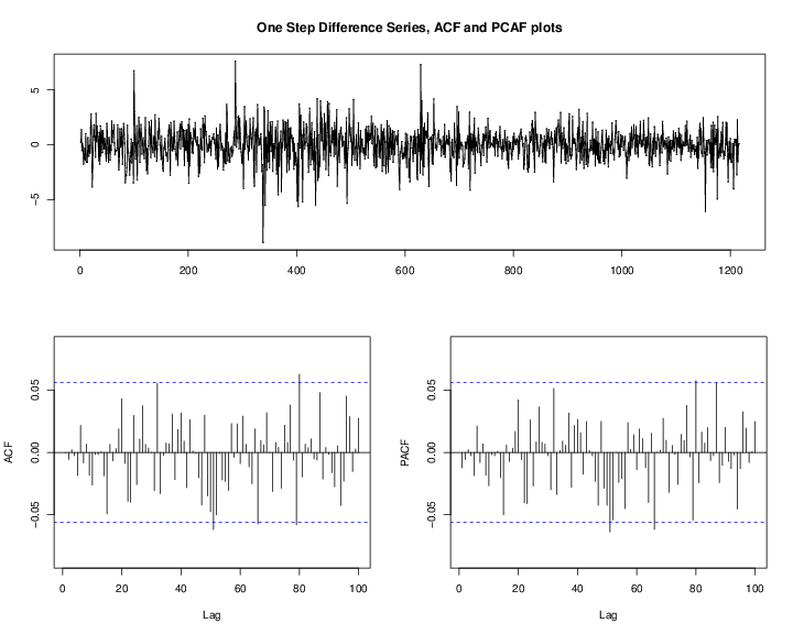
shown in Figure 7↓. Notice that there is almost none significant spike in ACF and PACF of Figure 7↓ and then we gave the result of following time series models.
2.1.1 Random Walk
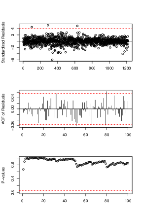
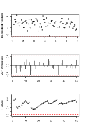
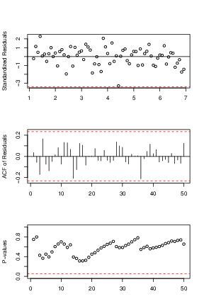
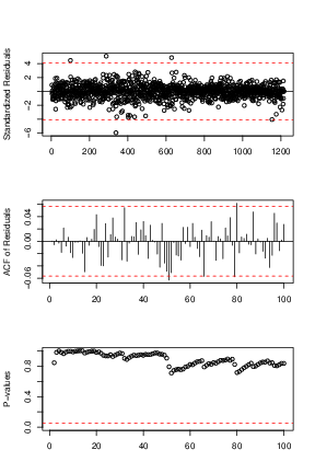
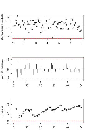
Because the best known example of unit-root nonstationary time series is the random walk model, our first linear model is random walk without drift (the mean constant). The point forecasts of a random-walk model are simply the value of the series at the forecast origin adding with the expectation of the error term (0 in this case). Our models for daily and monthly oil price are in Eq (↓) and (↓). The diagnostic plots can be referred by Figures a↓ and b↓ where we can see that the residuals of the fitted models are centered around
axis horizontal line, that they are uncorrelated with each others except some minor spikes in the ACF plots and that all the lags of the residuals pass the Box-Ljung test. Since the residuals are iid and satisfy the normality assumption, our random walk model here is valid and reasonable.
A second random walk model is to take the drift term into consideration or
and our fitted models for Daily and Monthly are in Eq (↓) and (↓). The diagnostics plots can be referred by Figures a↓ and b↓ where we can verify the model is valid using the similar argument as the above.
Since our fitting function arima use maximum likelihood for parameter estimations, the coefficients are asymptotically normal. Thus dividing the coefficients by their standard errors will give the
statistics. Then we can use the
statistics to calculate the drift’s significance. However both the drifts here are not significance. We can confirm that insignificance by almost identical diagnostic plots and forecasting values between the two models.
2.1.2 ARIMA
The second type of linear model is ARIMA. We tried many arima models such as
,
,
,
etc. according to the ACF and PCAF of Figure 7↓, but nailed down to
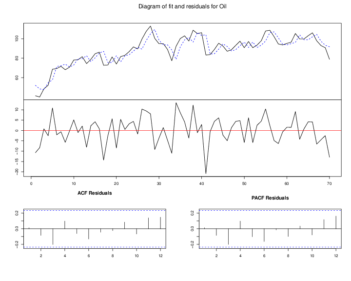
because it passes all the diagnostics test shown in Figure (10↓) and has the smallest AIC. The models for Daily and Monthly are Eq (↓) and (↓) respectively.
Again using
test statistics, the auto regressive parameters are not significant which is confirmed by the almost identical forecasting result and the diagnostics plots.
2.1.3 VAR
When building multiple linear regression models, one needs to take the collinearity issues into consideration where two or more predictor variables in the model are highly correlated. We tried to alleviate the problem by pairwise regressing the oil price with another explanatory variable such as gold price, SP500 index. After detecting the pool of significant variables, we then include them step by step and use smallest AIC to select the optimal models. The Table 1↓ and 2↓ show the significant levels for the explanatory variables. We can see that the weighted exchange rate (WEXC) and European and US exchange rate (EU-US EXC) are significant to the daily oil price and the order of significance from the least to the most for monthly oil price are gold price (Gold), unemployment rate (UNEMPR), weighted exchange rate (WEXC), total employment in oil mining (EMP), CPI energy index (CPIE). The optimal daily VAR model is regression of the oil price on weighted exchange rate but the model doesn’t pass the diagnostic test. The optimal monthly VAR model is regression of the oil price on WEXC, EMP, CPIE, and UEMPR whose diagnostics plot is shown in Figure 11↓.
2.2 Non Linear Models
The goal of time series prediction is to estimate some future value based on current and past data samples. We want to find a function
such that its estimation of the future point is unbiased and consistent. How about considering
as a non linear function? In this section, we introduced three famous types of non-linear models namely Support Vector Regression (SVR), Multiple Layer Perception (MLP) and Extreme Learning Machine (ELM).
The basic idea of SVR, MLP and ELM are the same. They all want to map the data
to a much higher dimension “feature” space by some activation function
where
.
2.2.1 SVR
The SVM is originally purposed for classification problem and it maps the data from the input space to some feature space
through some nonlinear Prior mapping function
. In this feature space, constraint optimization is used to find the “optimal” separating hyperplane that maximize the separating margins of two classifies in the feature space. Given a set of training data points
where
,
and
. We can mapped the training data point in the input space to some feature space
via a nonlinear function
. Then the distance between two hyperplane in the feature space
is
. We maximize the distance by minimizing its inverse or
After changing the Hinge loss function to Vapnik’s
-insensitive loss function in Eq (↓), SVM becomes SVR.
By Lagrange dual form and Mercer’s representation, SVR’s kernel form is
We used the Gaussian Kernel with the parameters selected by 10 folds cross validation.
2.2.2 MLP and ELM
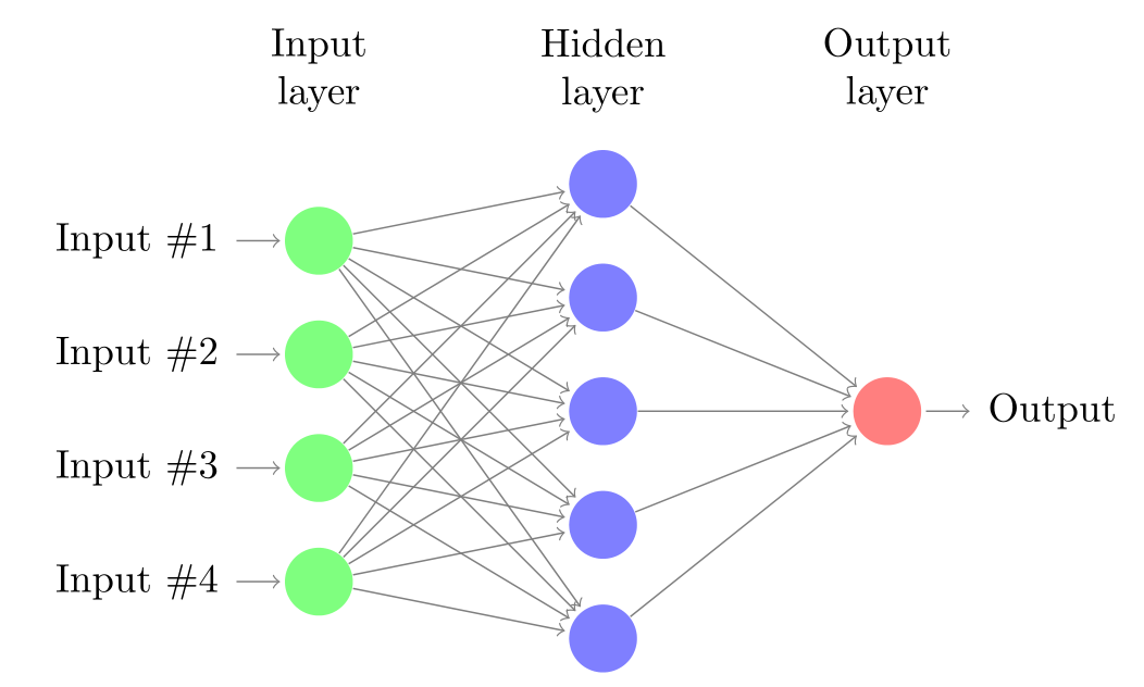
The MLP and ELM are both neural network (In our case we constraint hidden layer of MLP to 1 for comparison purpose.) and the architecture of the networks are shown in Figure 2↓. The activation function
used here is the sigmoid function. The only difference between ELM and MLP is that ELM doesn’t iteratively tune the activation functions’ parameters in the first layer and fixes those parameters once randomly generated. Or ELM randomly maps
to higher dimension space
as Eq (↓) and do a linear regression in the 2nd layer.
Its analytical solution is
where
and mapped space dimension
are user specified. Again by Mercer’s representation, we can map the original data to the kernel space whose dimension is equal to the training size. In our case, we used Gaussian kernel and the kernel parameters
and
are tuned using 10 folds cross validation.
MLP uses forward and backward propagation to tune the parameters in the first and second layers. Here we used caret package’s train function to build the MLP model.
2.3 Performance Comparison
2.3.1 Error metrics
The following
step ahead forecasting errors metrics where
are considered:
Root Mean Square Error (RMSE)
Mean Absolute Deviation (MAD)
Mean Absolute Percentage Error (MAPE)
2.3.2 Forecasting Accuracy Comparison
From Table 1↑ and 2↑, we can see that non-linear models performs better than linear models with different error metrics and ELM has the smallest prediction error compared to other methods. Please refer to Figure 12↓ and Figure 13↓ to see how accurate those models forecast compared to the true oil prices.
3 Oil Volatility Forecasting
3.1 Model Selection
In this section we analyzed the volatility of oil price through ARCH and GARCH models. We used daily oil spot prices from 2010-01-01 to 2014-10-28. The price series were converted to logarithmic returns:
for
where
denotes as the log returns for each crude oil price at time
and
as the oil price. Figure 3↓ below shows the dynamics of log returns and its ACF plot.
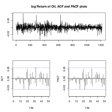
From the ACF plot of Figure a↑, there is no significant serial correlations except some minor ones. Therefore we can apply the mean equation:
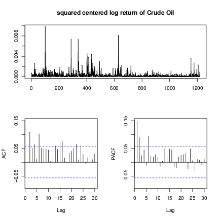
. Then we performed a Ljung-Box test on squared centered returns
where
on lags 6 and 10. The P values are 1.348e-11 and 8.715e-12, which are less than the 0.05 significant level. Therefore we can conclude that there exists strong ARCH effects.
We used the PACF of the squared centered returns
in Figure b↑ to determine the ARCH order. Since the lags cut off at 2 and 6, we tried the
and
. We also applied
and
models. Finally we chose
because it is not only the simplest model but also has smaller AIC than
.
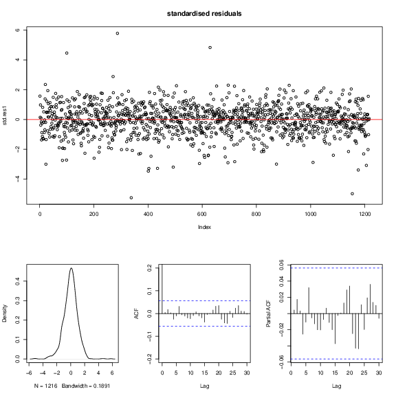
3.2 Model Diagnostics
To check the adequacy of our model
, we took a look at the standardized residual test. Because the Ljung-Box test of standardized residuals gives p-values larger than 0.05 for both standardized residuals and squared standardized residuals, therefore both the mean equation and volatility equation are adequate. In Figure 4↓, the standardized residuals spread randomly and symmetric over x-axis. For ACF and PACF plots there are not significant serial correlations. However, the residuals are slightly skewed to the left in the density plot.
3.3 Model Forecasting Comparison
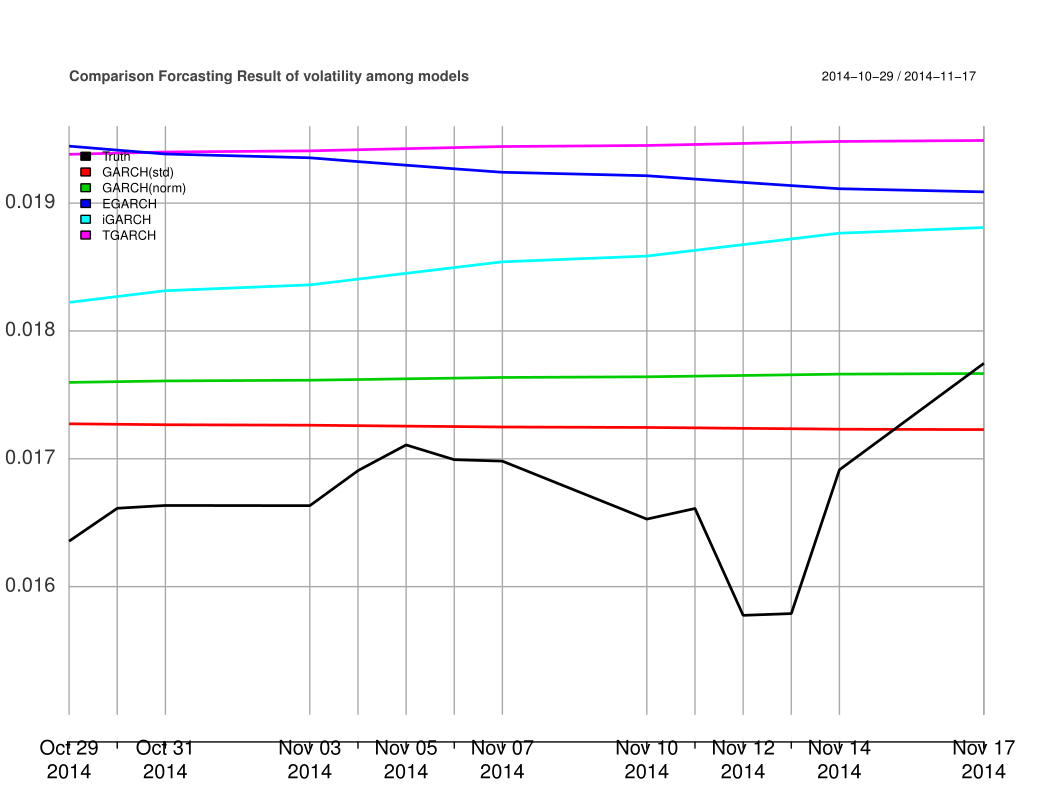
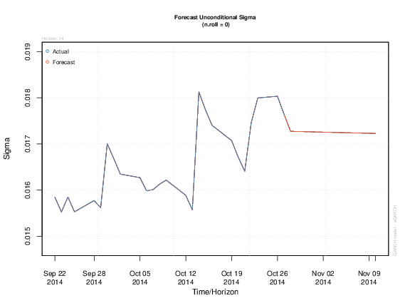
Finally we analyzed the volatility forecasting accuracy of GARCH-type models. In the order (1,1), we applied GARCH family models with student-t distribution and normal distribution, exponential GARCH model, integrated GARCH model and Threshold GARCH model. We utilized these models to predict the volatility from 2014-10-29 to 2014-11-17 (14 steps ahead). We used a time window of 30 days to compute the true volatility from 2010-01-01 to 2014-11-17.
From Table 5↑, it is obvious that the
with student-t distribution has the best forecasting accuracy with the smallest errors. In Figure 4, we compared the forecasting performance of these GARCH-type models in term of accuracy. The black line indicates the true sigma. It is interesting to note that at the last day of the prediction period (2014-11-17), the forecasting from GARCH(1,1) with normal distribution (the gray line) approximates well to the real sigma. However, the red line (GARCH with student-t distribution) is the closest approach to the real volatility. According to the error matrix Table 5↑, we can come out with the conclusion that among these models, GARCH(1,1) with student-t distribution is the best in oil price volatility forecasting.
4 Conclusion
In this project, we analyzed various time series models on the oil price and volatility forecasting. For the price prediction part, we grouped our forecasting methods into the two major categories: linear and non-linear. The linear models we applied are random walk with and without drift,
and VAR. According to our VAR models, the oil price has significant correlation with CPIE, exchange currency, unemployment rate but little correlation with the gold price. We further utilized the 3 non-linear models SVR, MLP and ELM for oil price forecasting. In term of forecasting accuracy, all non-linear models win over the linear ones and ELM is the best model. For the volatility forecasting part, we first explored the
and
family and selected their optimal models using minimum AIC. We finally picked
with
innovations as the best model for its smallest forecasting errors among the other models.
\newpage